PCA for industrial diagnostic of compressor connection rod defects

PROBLEM DESCRIPTION: Industrial production of compressors suffers from problems during the imprinting operation where a connection rod is connected with a compressor head. Irregular imprinting can cause damage or crack of the connection rod which results in damaged compressor. Such compressors should be eliminated from the production line but defects of this type are difficult to detect. The task is to detect crack and overload defects from the measurement of the imprinting force.

Photos of the broken connection rod
Load and plot data
Prepare inputs by PCA
Define output coding: 0=OK, 1=Error
Create and train a multilayer perceptron
Evaluate network performance
Plot classification result

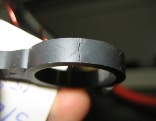
Photos of the broken connection rod

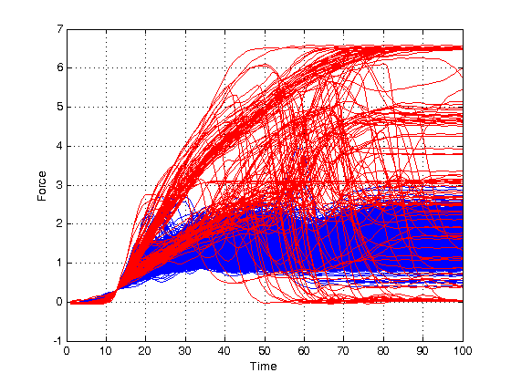
Load and plot data

close all, clear all, clc, format compact

% industrial data
load data2.mat
whos

% show data
figure
plot(force(find(target==1),:)','b') % OK (class 1)
grid on, hold on
plot(force(find(target>1),:)','r') % NOT OK (class 2 & 3)
xlabel('Time')
ylabel('Force')

  Name           Size               Bytes  Class     Attributes

  force       2000x100            1600000  double              
  notes          1x3                  222  cell                
  target      2000x1                16000  double

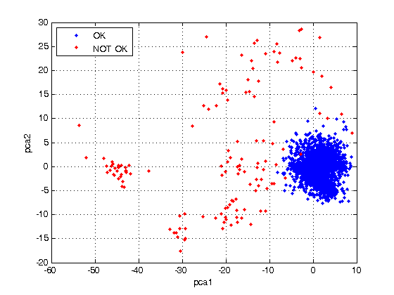
Prepare inputs by PCA

% 1. Standardize inputs to zero mean, variance one
[pn,ps1] = mapstd(force');

% 2. Apply Principal Compoments Analysis
% inputs whose contribution to total variation are less than maxfrac are removed
FP.maxfrac = 0.1;
% process inputs with principal component analysis
[ptrans,ps2] = processpca(pn, FP);
ps2
% transformed inputs
force2 = ptrans';
whos force force2

% plot data in the space of first 2 PCA components
figure
plot(force2(:,1),force2(:,2),'.') % OK
grid on, hold on
plot(force2(find(target>1),1),force2(find(target>1),2),'r.') % NOT_OK
xlabel('pca1')
ylabel('pca2')
legend('OK','NOT OK','location','nw')

% % plot data in the space of first 3 PCA components
% figure
% plot3(force2(find(target==1),1),force2(find(target==1),2),force2(find(target==1),3),'b.')
% grid on, hold on
% plot3(force2(find(target>1),1),force2(find(target>1),2),force2(find(target>1),3),'r.')

ps2 = 
         name: 'processpca'
        xrows: 100
      maxfrac: 0.1000
        yrows: 2
    transform: [2x100 double]
    no_change: 0
  Name           Size               Bytes  Class     Attributes

  force       2000x100            1600000  double              
  force2      2000x2                32000  double

Define output coding: 0=OK, 1=Error

% binary coding 0/1
target = double(target > 1);

Create and train a multilayer perceptron

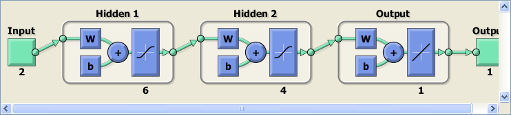
% create a neural network
net = feedforwardnet([6 4]);

% set early stopping parameters
net.divideParam.trainRatio = 0.70; % training set [%]
net.divideParam.valRatio   = 0.15; % validation set [%]
net.divideParam.testRatio  = 0.15; % test set [%]

% train a neural network
[net,tr,Y,E] = train(net,force2',target');

% show net
view(net)

Evaluate network performance

% digitize network response
threshold = 0.5;
Y = double(Y > threshold)';

% find percentage of correct classifications
cc = 100*length(find(Y==target))/length(target);
fprintf('Correct classifications: %.1f [%%]\n', cc)

Correct classifications: 99.6 [%]

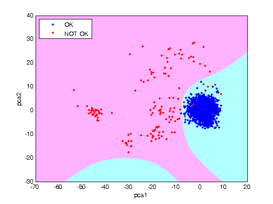
Plot classification result

figure(2)
a = axis;
% generate a grid, expand input space
xspan = a(1)-10 : .1 : a(2)+10;
yspan = a(3)-10 : .1 : a(4)+10;
[P1,P2] = meshgrid(xspan,yspan);
pp      = [P1(:) P2(:)]';
% simualte neural network on a grid
aa      = sim(net,pp);
aa      = double(aa > threshold);

% plot classification regions based on MAX activation
ma = mesh(P1,P2,reshape(-aa,length(yspan),length(xspan))-4);
mb = mesh(P1,P2,reshape( aa,length(yspan),length(xspan))-5);
set(ma,'facecolor',[.7 1.0 1],'linestyle','none');
set(mb,'facecolor',[1 0.7  1],'linestyle','none');
view(2)