Bayesian regularization for RBFN
Neural Networks course (practical examples) © 2012 Primoz Potocnik
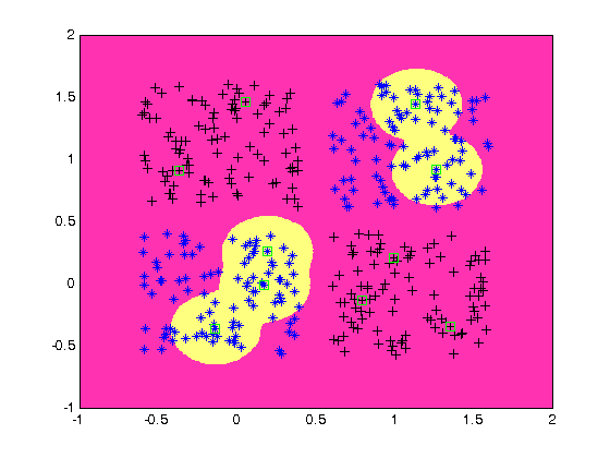
PROBLEM DESCRIPTION: 2 groups of linearly inseparable data (A,B) are defined in a 2-dimensional input space. The task is to define a neural network for solving the XOR classification problem.
Contents
- Create input data
- Define output coding
- Prepare inputs & outputs for network training
- Create a RBFN
- Evaluate network performance
- Plot classification result
- Retrain a RBFN using Bayesian regularization backpropagation
- Evaluate network performance after Bayesian regularization training
- Plot classification result after Bayesian regularization training
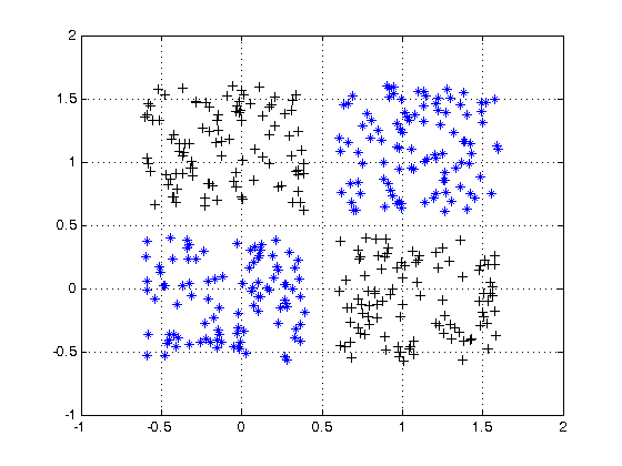
Create input data
close all, clear all, clc, format compact

% number of samples of each cluster
K = 100;
% offset of clusters
q = .6;
% define 2 groups of input data
A = [rand(1,K)-q rand(1,K)+q;
     rand(1,K)+q rand(1,K)-q];
B = [rand(1,K)+q rand(1,K)-q;
     rand(1,K)+q rand(1,K)-q];
% plot data
plot(A(1,:),A(2,:),'k+',B(1,:),B(2,:),'b*')
grid on
hold on
Define output coding
% coding (+1/-1) for 2-class XOR problem
a = -1;
b =  1;
Prepare inputs & outputs for network training
% define inputs (combine samples from all four classes)
P = [A B];
% define targets
T = [repmat(a,1,length(A)) repmat(b,1,length(B))];
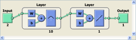
Create a RBFN
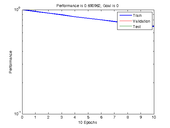
% choose a spread constant
spread = .1;
% choose max number of neurons
K      = 10;
% performance goal (SSE)
goal   = 0;
% number of neurons to add between displays
Ki     = 2;
% create a neural network
net    = newrb(P,T,goal,spread,K,Ki);

% view network
view(net)
NEWRB, neurons = 0, MSE = 1
NEWRB, neurons = 2, MSE = 0.928277
NEWRB, neurons = 4, MSE = 0.855829
NEWRB, neurons = 6, MSE = 0.798564
NEWRB, neurons = 8, MSE = 0.742854
NEWRB, neurons = 10, MSE = 0.690962
Evaluate network performance
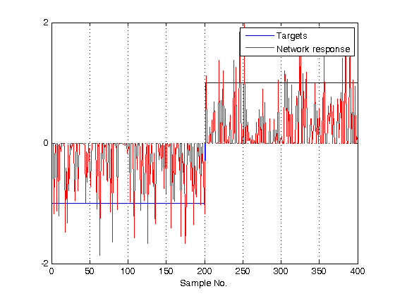
% check RBFN spread
actual_spread = net.b{1}

% simulate RBFN on training data
Y = net(P);

% calculate [%] of correct classifications
correct = 100 * length(find(T.*Y > 0)) / length(T);
fprintf('\nSpread          = %.2f\n',spread)
fprintf('Num of neurons  = %d\n',net.layers{1}.size)
fprintf('Correct class   = %.2f %%\n',correct)

% plot targets and network response to see how good the network learns the data
figure;
plot(T')
ylim([-2 2])
set(gca,'ytick',[-2 0 2])
hold on
grid on
plot(Y','r')
legend('Targets','Network response')
xlabel('Sample No.')
actual_spread =
    8.3255
    8.3255
    8.3255
    8.3255
    8.3255
    8.3255
    8.3255
    8.3255
    8.3255
    8.3255

Spread          = 0.10
Num of neurons  = 10
Correct class   = 79.50 %
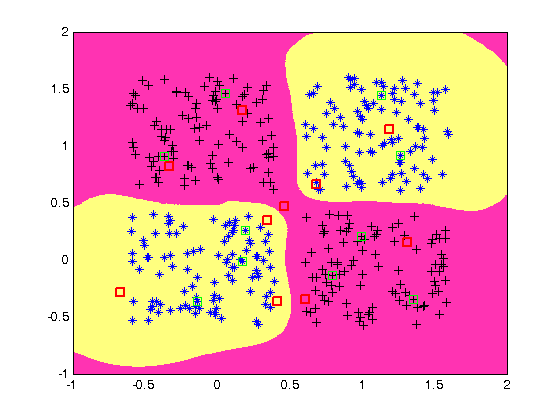
Plot classification result
% generate a grid
span    = -1:.025:2;
[P1,P2] = meshgrid(span,span);
pp      = [P1(:) P2(:)]';
% simualte neural network on a grid
aa      = sim(net,pp);

% plot classification regions based on MAX activation
figure(1)
ma = mesh(P1,P2,reshape(-aa,length(span),length(span))-5);
mb = mesh(P1,P2,reshape( aa,length(span),length(span))-5);
set(ma,'facecolor',[1 0.2 .7],'linestyle','none');
set(mb,'facecolor',[1 1.0 .5],'linestyle','none');
view(2)

% plot RBFN centers
plot(net.iw{1}(:,1),net.iw{1}(:,2),'gs')
Retrain a RBFN using Bayesian regularization backpropagation
% define custom training function: Bayesian regularization backpropagation
net.trainFcn='trainbr';
% perform Levenberg-Marquardt training with Bayesian regularization
net = train(net,P,T);
Evaluate network performance after Bayesian regularization training
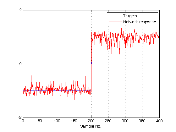
% check new RBFN spread
spread_after_training = net.b{1}
% simulate RBFN on training data
Y = net(P);

% calculate [%] of correct classifications
correct = 100 * length(find(T.*Y > 0)) / length(T);
fprintf('Num of neurons  = %d\n',net.layers{1}.size)
fprintf('Correct class   = %.2f %%\n',correct)

% plot targets and network response
figure;
plot(T')
ylim([-2 2])
set(gca,'ytick',[-2 0 2])
hold on
grid on
plot(Y','r')
legend('Targets','Network response')
xlabel('Sample No.')
spread_after_training =
    2.9924
    3.0201
    0.7809
    0.5933
    2.6968
    2.8934
    2.2121
    2.9748
    2.7584
    3.5739
Num of neurons  = 10
Correct class   = 100.00 %
Plot classification result after Bayesian regularization training
% simulate neural network on a grid
aa = sim(net,pp);
% plot classification regions based on MAX activation
figure(1)
ma = mesh(P1,P2,reshape(-aa,length(span),length(span))-5);
mb = mesh(P1,P2,reshape( aa,length(span),length(span))-5);
set(ma,'facecolor',[1 0.2 .7],'linestyle','none');
set(mb,'facecolor',[1 1.0 .5],'linestyle','none');
view(2)

% Plot modified RBFN centers
plot(net.iw{1}(:,1),net.iw{1}(:,2),'rs','linewidth',2)