ADALINE time series prediction

Neural Networks course (practical examples) © 2012 Primoz Potocnik

PROBLEM DESCRIPTION: Construct an ADALINE for adaptive prediction of time series based on past time series data

Contents

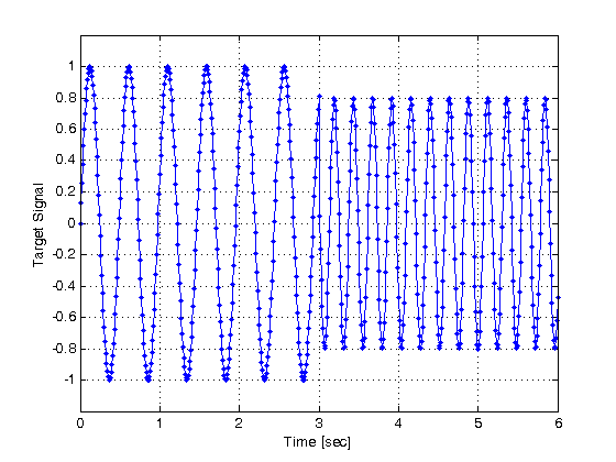
Define input and output data

close all, clear all, clc, format compact

% define segments of time vector
dt = 0.01; % time step [seconds]
t1 = 0    : dt : 3; %    first time vector [seconds]
t2 = 3+dt : dt : 6; %   second time vector [seconds]
t = [t1 t2];        % complete time vector [seconds]
% define signal
y = [sin(4.1*pi*t1) .8*sin(8.3*pi*t2)];
% plot signal
plot(t,y,'.-')
xlabel('Time [sec]');
ylabel('Target Signal');
grid on
ylim([-1.2 1.2])

Prepare data for neural network toolbox

% There are two basic types of input vectors: those that occur concurrently
% (at the same time, or in no particular time sequence), and those that
% occur sequentially in time. For concurrent vectors, the order is not
% important, and if there were a number of networks running in parallel,
% you could present one input vector to each of the networks. For
% sequential vectors, the order in which the vectors appear is important.
p = con2seq(y);

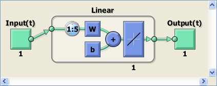
Define ADALINE neural network

% The resulting network will predict the next value of the target signal
% using delayed values of the target.
inputDelays   = 1:5; % delayed inputs to be used
learning_rate = 0.2; % learning rate

% define ADALINE
net = linearlayer(inputDelays,learning_rate);

Adaptive learning of the ADALINE

% Given an input sequence with N steps the network is updated as follows.
% Each step in the sequence of  inputs is presented to the network one at
% a time.  The network's weight and bias values are updated after each step,
% before the next step in the sequence is presented. Thus the network is
% updated N times. The output signal and the error signal are returned,
% along with new network.
[net,Y,E] = adapt(net,p,p);

% view network structure
view(net)

% check final network parameters
disp('Weights and bias of the ADALINE after adaptation')
net.IW{1}
net.b{1}

Weights and bias of the ADALINE after adaptation
ans =
    0.7179    0.4229    0.1552   -0.1203   -0.4159
ans =
  -1.2520e-08

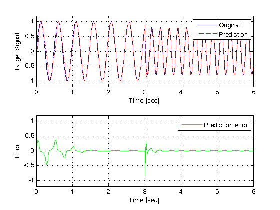
Plot results

% transform result vectors
Y = seq2con(Y); Y = Y{1};
E = seq2con(E); E = E{1};
% start a new figure
figure;

% first graph
subplot(211)
plot(t,y,'b', t,Y,'r--');
legend('Original','Prediction')
grid on
xlabel('Time [sec]');
ylabel('Target Signal');
ylim([-1.2 1.2])

% second graph
subplot(212)
plot(t,E,'g');
grid on
legend('Prediction error')
xlabel('Time [sec]');
ylabel('Error');
ylim([-1.2 1.2])

Published with MATLAB® 7.14